Programming – Page 3 – Montessori Muddle

Headless Pi Zero

Pi Zero‘s are even cheaper versions of the Raspberry Pi. The price you pay is that they’re harder to connect to since all the ports are small (micro-USB’s and mini-HDMI’s), so you need adapters to connect to keyboards, mice, and monitors. However, if you have the wireless version (Pi Zero W) you can set it up to automatically connect to the WiFi network, and work on it through there using the command line. This is a brief summary of how to do this (it’s called a “headless” setup) based on Taron Foxworth’s instructions. It should work for the full Raspberry Pi as well.

Set up the Operating System

You can install the Raspbian Stretch (or Raspbian Lite which does not include the desktop GUI that you will not use) on a SD card (I used 8 or 16 Gb cards).

Download Raspbian.
SD Card Formatter to format the SD Card. It’s pretty quick, just follow the instructions.
Etcher: to install the operating system on the SD Card

Set up automatic connection to WiFi

You may have to remove and reinsert the SD Card to get it to show up on the file system, but once you have you can set it up to automatically connect to WiFi by:

Go into the /boot partition (it usually shows up as the base of the SD Card on your file manager) and create a file named “ssh”.
Create a text file called “wpa_supplicant.conf” in the /boot folder, and put the following into it, assuming that the wifi router you’re connecting to is called “myWifi” and the password is “myPassword”.

country=US
ctrl_interface=DIR=/var/run/wpa_supplicant GROUP=netdev
update_config=1

network={
 ssid="myWifi"
 scan_ssid=1
 psk="myPassword"
 key_mgmt=WPA-PSK
}

Now put the SD Card into the Pi and plug in the power.

Find the IP address

First you have to find the Pi on the local network. On Windows I use Cygwin to get something that looks and acts a bit like a unix terminal (on Mac you can use Terminal, or any shell window on Linux).

To find the ip address of your local network use:

on Windows:

> ipconfig

look for the “IPv4 Address”.

Mac (and Linux?)

> ifconfig

look under “en1:”

Connecting

To connect you use ssh on the command line (Mac or Linux) or something like Putty

Static IP

Without a static IP address it is possible that the Pi’s IP address will change occasionally. I followed the instructions on Circuit Basics and MODMYPI, but basically you have to:

Identify your network information:

Find your Gateway:

> route -ne

Find your Domain Server:

> cat /etc/resolv.conf

Add the information to the end of your /etc/dhcpcd.conf file (here the wlan0 means you’re doing this to the wireless interface (WiFi) and the static ip is 10.0.0.99, the static router the gateway ip you found above, and the domain_name_servers takes the domain server ip):

interface wlan0
static ip_address=10.0.0.99
static routers=10.0.0.1
static domain_name_servers=75.75.75.75

Now reboot and you should be able to ssh or sftp into the new static IP.

A Web Server

Adding a webserver (apache with php) is pretty easy as well, just run the commands (from the Raspberry Pi Foundation)

Apache web server:

sudo apt-get install apache2 -y

PHP for server-side scripting

sudo apt-get install php libapache2-mod-php -y

Now your can find the webpage by going to the ip address (e.g. http://10.0.0.1).

The actual file that you’re seeing is located on the Pi at:

/var/www/html/index.html

You will probably need to change the ownership of the file in order to edit it by running:

> sudo chown pi: index.html

A Really Quick Introduction to Programming

With examples using python.

Statement: A command given to the computer.

Assign a value of -9.8 to a variable called “g”:

g = -9.8

Print the value of “g” to the screen:

print g

Variable: A placeholder name used to record data for later use. In the first statement above, g, is a variable and it is assigned a value of -9.8. Variable names in python start with a letter or underscore “_”. Variables can hold different types of data, for example:

strings:

x = "hello"

Floating point number (aka. a float):

x = 9.8

Integer:

x = 5

True/False (aka boolean):

x = True

Operations: Statements where some sort of calculation is made:

Add two numbers and assign the result to a variable called “y”:

y = 3 + 5

Divide the value in the variable “y” by 2 and then assign the value to another variable called “z”:

z = y / 2

Operators: The symbols that tell what operation to do:

+ – * / are used for addition, subtraction, multiplication, and division respectively
** is used for exponents so 5 squared (5²) is:

a = 5**2

Loops: Tell the computer to do something over and over again. There are different types:

“For” loops are good for doing things a set number of times

for i in range(5):
	print i

results in:

Logical statements: These test to see if something is True or False and then do different things based on the outcome:

Assign a value to a variable called “x”, check to see if the value is greater than 10, and print out a different sentence based on the result:

x = 12
if (x > 10):
	print "x is greater than 10"
else:
	print "x is less than 10"

Functions: Chunks of code that someone (maybe even you) wrote that can be referenced via a shortcut:

def forceOfGravity(mass):
	Fg = mass * -9.8
	return Fg

Call the function to find the force of gravity acting on a mass of 100 kg and print out the result:

x = forceOfGravity(100)
print x

the result should be:

-980

Classes: A class is like a function that you can assign to a variable and then have it do a lot more stuff.

from visual import *
ball = sphere()
ball.color = color.red

Hour of Code

We are trying the Hour of Code today. Updates to follow.

How to Build an 8-bit Computer on a Breadboard

Ben Eater’s excellent series on building a computer from some basic components. It goes how things work from the transistors to latches and flip-flops to the architecture of the main circuits (clock, registers etc). The full playlist.

Other good resources include:

Nand2Tetris : Building a computer from first principles (this one uses a hardware simulator however): See overview video.

Modeling Earth’s Energy Balance (Zero-D) (Transient)

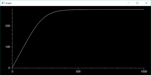
Temperature change over time (in thousands of years). As the Earth warms from 3K to equilibrium.

If the Earth behaved as a perfect black body and absorbed all incoming solar radiation (and radiated with 100% emissivity) the we calculated that the average surface temperature would be about 7 degrees Celsius above freezing (279 K). Keeping with this simplification we can think about how the Earth’s temperature could change with time if it was not at equilibrium.

If the Earth started off at the universe’s background temperature of about 3K, how long would it take to get up to the equilibrium temperature?

Using the same equations for incoming solar radiation (E_in) and energy radiated from the Earth (E_out):

$E_{in} = I \times \pi (r_E)^2$

$E_{out} = \sigma T^4 4 \pi r_{E}^2$

Symbols and constants are defined here except:

r_E = 6.371 x 10⁶ m

At equilibrium the energy in is equal to the energy out, but if the temperature is 3K instead of 279K the outgoing radiation is going to be a lot less than at equilibrium. This means that there will be more incoming energy than outgoing energy and that energy imbalance will raise the temperature of the Earth. The energy imbalance (ΔE) would be:

$\Delta E = E_{in}-E_{out}$

All these energies are in Watts, which as we’ll recall are equivalent to Joules/second. In order to change the temperature of the Earth, we’ll need to know the specific heat capacity (c_E) of the planet (how much heat is required to raise the temperature by one Kelvin per unit mass) and the mass of the planet. We’ll approximate the entire planet’s heat capacity with that of one of the most common rocks, granite. The mass of the Earth (m_E) we can get from NASA:

c_{E = 800 J/kg/K}
m_E = 5.9723×10²⁴kg

So looking at the units we can figure out the the change in temperature (ΔT) is:

$\Delta T = \frac{\Delta E \Delta t}{c_E m_E}$

Where Δt is the time step we’re considering.

Now we can write a little program to model the change in temperature over time:

EnergyBalance.py

from visual import *
from visual.graph import *

I = 1367.
r_E = 6.371E6
c_E = 800.
m_E = 5.9723E24

sigma = 5.67E-8

T = 3                               # initial temperature

yr = 60*60*24*365.25
dt = yr * 100
end_time = yr * 1000000
nsteps = int(end_time/dt)

Tgraph = gcurve()

for i in range(nsteps):
    t = i*dt
    E_in = I * pi * r_E**2
    E_out = sigma * (T**4) * 4 * pi * r_E**2
    dE = E_in - E_out
    dT = dE * dt / (c_E * m_E)
    T += dT
    Tgraph.plot(pos=(t/yr/1000,T))
    if i%10 == 0:
        print t/yr, T
        rate(60)

The results of this simulation are shown at the top of this post.

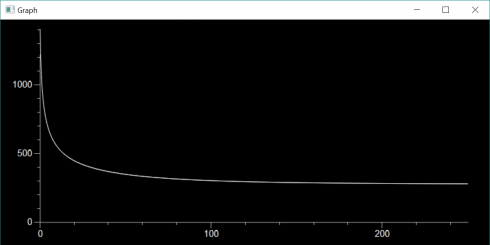
What if we changed the initial temperature from really cold to really hot? When the Earth formed from the accretionary disk of the solar nebula the surface was initially molten. Let’s assume the temperature was that of molten granite (about 1500K).

Cooling if the Earth started off molten (1500K). Note that this simulation only runs for 250,000 years, while the warming simulation (top of page) runs for 1,000,000 years.

Modeling Earth’s Energy Balance (Zero-D) (Equilibrium)

For conservation of energy, the short-wave solar energy absorbed by the Earth equals the long-wave outgoing radiation.

Energy and matter can’t just disappear. Energy can change from one form to another. As a thrown ball moves upwards, its kinetic energy of motion is converted to potential energy due to gravity. So we can better understand systems by studying how energy (and matter) are conserved.

Energy Balance for the Earth

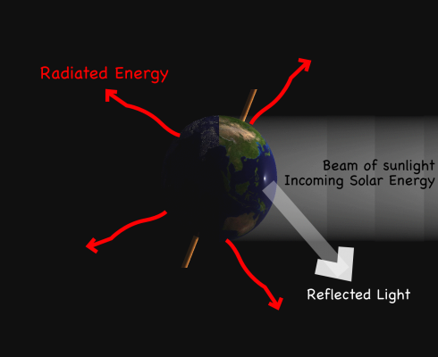
Let’s start by considering the Earth as a simple system, a sphere that takes energy in from the Sun and radiates energy off into space.

Incoming Energy

At the Earth’s distance from the Sun, the incoming radiation, called insolation, is 1367 W/m². The total energy (wattage) that hits the Earth (E_in) is the insolation (I) times the area the solar radiation hits, which is the area a cross section of the Earth (A_cx).

$E_{in} = I \times A_{cx}$

Given the Earth’s radius (r_E) and the area of a circle, this becomes:

$E_{in} = I \times \pi (r_E)^2$

Outgoing Energy

The energy radiated from the Earth is can be calculated if we assume that the Earth is a perfect black body–a perfect absorber and radiatior of Energy (we’ve already been making this assumption with the incoming energy calculation). In this case the energy radiated from the planet (E_out) is proportional to the fourth power of the temperature (T) and the surface area that is radiated, which in this case is the total surface area of the Earth (A_surface):

$E_{out} = \sigma T^4 A_{surface}$

The proportionality constant (σ) is: σ = 5.67 x 10^-8 W m^-2 K^-4

Note that since σ has units of Kelvin then your temperature needs to be in Kelvin as well.

Putting in the area of a sphere we get:

$E_{out} = \sigma T^4 4 \pi r_{E}^2$

Balancing Energy

Now, if the energy in balances with the energy out we are at equilibrium. So we put the equations together:

$E_{in} = E_{out}$

$I \times \pi r_{E}^2 = \sigma T^4 4 \pi r_{E}^2$

cancelling terms on both sides of the equation gives:

$I = 4 \sigma T^4$

and solving for the temperature produces:

$T = \sqrt{\frac{I}{4 \sigma}}$

Plugging in the numbers gives an equilibrium temperature for the Earth as:

T = 278.6 K

Since the freezing point of water is 273K, this temperature is a bit cold (and we haven’t even considered the fact that the Earth reflects about 30% of the incoming solar radiation back into space). But that’s the topic of another post.

Projectile Paths

Paths of a projectile. The half oval represents a line connecting the maximum heights of each projectile. — Paths of a projectile.

I had my Numerical Methods student calculate the angle that would give a ballistic projectile its maximum range, then I had them write a program that did the the same by just trying a bunch of different angles. The diagram above is what they came up with.

It made an interesting pattern that I converted into a face-plate cover for a light switch that I made using the laser at the TechShop.

Maximum Range of a Potato Gun

One of the middle schoolers built a potato gun for his math class. He was looking a the mathematical relationship between the amount of fuel (hair spray) and the hang-time of the potato. To augment this work, I had my Numerical Methods class do the math and create analytical and numerical models of the projectile motion.

One of the things my students had to figure out was what angle would give the maximum range of the projectile? You can figure this out analytically by finding the function for how the horizontal distance (x) changes as the angle (theta) changes (i.e. x(theta)) and then finding the maximum of the function.

Initial velocity vector (v) and its component vectors in the x and y directions. — Initial velocity vector (v) and its component vectors in the x and y directions for a given angle.

Distance as a function of the angle

In a nutshell, to find the distance traveled by the potato we break its initial velocity into its x and y components (v_x and v_y), use the y component to find the flight time of the projectile (t_f), and then use the v_x component to find the distance traveled over the flight time.

Starting with the diagram above we can separate the initial velocity of the potato into its two components using basic trigonometry:

$\cos{\theta} = \frac{v_x}{v}$
$\sin{\theta} = \frac{v_y}{v}$ ,

so,

$v_x = v \cos{\theta}$ ,
$v_y = v \sin{\theta}$

Now we know that the height of a projectile (y) is given by the function:

$! y(t) = \frac{a t^2}{2} + v_0 t + y_0$

(you can figure this out by assuming that the acceleration due to gravity (a) is constant and acceleration is the second differential of position with respect to time.)

To find the flight time we assume we’re starting with an initial height of zero (y₀ = 0), and that the flight ends when the potato hits the ground which is also at zero ((y_t = 0), so:

$! 0 = \frac{a t^2}{2} + v_0 t + 0$

$! 0 = \frac{a t^2}{2} + v_0 t$

Factoring out t gives:

$! 0 = t ( \frac{a t}{2} + v_0)$

Looking at the two factors, we can now see that there are two solutions to this problem, which should not be too much of a surprise since the height equation is parabolic (a second order polynomial). The solutions are when:

$! t = 0$

$! \frac{a t}{2} + v_0 = 0$

The first solution is obviously the initial launch time, while the second is going to be the flight time (t_f).

$! \frac{a t_f}{2} + v_0 = 0$

$! t_f = - \frac{2 v_0}{a}$

You might think it’s odd to have a negative in the equation, but remember, the acceleration is negative so it’ll cancel out.

Now since we’re working with the y component of the velocity vector, the initial velocity in this equation (v₀) is really just v_y:

$! v_0 = v_y$

so we can substitute in the trig function for v_y to get:

$! t_f = - \frac{2 v \sin{\theta}}{a}$

Our horizontal distance is simply given by the velocity in the x direction (v_x) times the flight time:

$! x = v_x t_f$

which becomes:

$! x = v_x \left(- \frac{2 v \sin{\theta}}{a}\right)$

and substituting in the trig function for v_x (just to make things look more complicated):

$! x = \left( v \cos{\theta} \right) \left(- \frac{2 v \sin{\theta}}{a}\right)$

and factoring out some of the constants gives:

$! x = -\frac{v^2}{a} 2 \sin{\theta}\cos{theta}$

Now we have distance as a function of the launch angle.

We can simplify this a little by using the double-angle formula:

$! \sin{2\theta} = 2 \sin{\theta}\cos{theta}$

to get:

$! x = -\frac{v^2}{a} \sin{2\theta}$

Finding the maximum distance

How do we find the maxima for this function. Sketching the curve should be easy enough, but because we know a little calculus we know that the maximum will occur when the first differential is equal to zero. So we differentiate with respect to the angle to get:

$! \frac{dx}{d\theta} = -\frac{v^2}{a} 2 \cos{2\theta}$

and set the differential equal to zero:

$! 0 = -\frac{v^2}{a} 2 \cos{2\theta}$

and solve to get:

$! \cos{2\theta} = 0$

$! 2\theta = \cos^{-1}{(0)}$

Since we remember that the arccosine of 0 is 90 degrees:

$! 2\theta = 90^{\circ}$

$! \theta = 45^{\circ}$

And thus we’ve found the angle that gives the maximum launch distance for a potato gun.