Tsunami Geometry: Calculating the Height of a Tsunami using Basic Geometry

Since we’re working on geometry this cycle, I thought it would be an interesting exercise to think about how we could use geometry to think about how the strength of tsunamis decreases with distance from the source.

Of course, we’ll have to do this using some intense simplification so we can actually apply the tools we have available. The first is to approximate the tsunami as a circular wall of water centered on the epicenter of the earthquake.

tsunami-geometry — Simplified tsunami geometry.

This lets us figure out the volume of the wave pretty easily because we know that the volume of a cylinder is:

(1) $! V_c = \pi r^2 h$

The size of the circular water wall we approximate from the reports from Japan. The maximum height of the wave at landfall was somewhere in the range of 14 m along the northern Japanese coast, which was about 80 km from the epicenter. Just as a wild guess, I’m assuming that the “effective” width of the wave is 1 km.

Typically, in deep water, a tsunami can have a wavelength greater than 500 km (Nelson, 2010; note that our width is half the wavelength), but a wave height of only 1 m (USSRTF). When they reach the shallow water the wave height increases. The Japanese tsunami’s maximum height was reportedly about 14 m.

At any rate, we can figure out the volume of our wall of water by calculating the volume of a cylinder with the middle cut out of it. The radius of our inner cylinder is 80 km, and the radius of the outer cylinder is 80 km plus the width of the wave, which we say here is 1 km.

Calculating the volume of the wave

However, for the sake of algebra, we’ll call the radius of the inner cylinder, r_i and the width of the wave as w. Therefore the inner cylinder has a volume of:

(2) $! V_i = \pi r_i^2 h$

So the radius of the outer cylinder is the radius of the inner cylinder plus the width of the wave:

(3) $! r_o = r_i + w$

which means that the volume of the outer cylinder is:

(4) $! V_o = \pi (r_i + w)^2 h$

So now we can figure out the volume of the wave, which is the volume of the outer cylinder minus the volume of the inner cylinder:

(5) $! V_w = V_o - V_i$

(6) $! V_w = \pi (r_i + w)^2 h - \pi r_i^2 h$

Now to simplify, let’s expand the first term on the right side of the equation:

(7) $! V_w = \pi (r_i ^2 + 2 r_i w + w^2) h - \pi r_i^2 h$

Now let’s collect terms:

(8) $! V_w = \pi h \left( (r_i ^2 + 2 r_i w + w^2) - r_i^2 \right)$

Take away the inner parentheses:

(9) $! V_w = \pi h (r_i ^2 + 2 r_i w + w^2 - r_i^2)$

and subtract similar terms to get the equation:

(10) $! V_w = \pi h ( 2 r_i w + w^2 )$

Volume of the wave

Now we can just plug in our estimates of width and height to get the volume of water in the wave. We’re going to assume, later on, that the volume of water does not change as the wave propagates across the ocean.

(11) $! V_w = \pi (14) ( 2 r_i (1000) + (1000)^2 )$

rearrange so the coefficients are in front of the variables:

(12) $! V_w = 14 \pi ( 2000 r_i + 1000000 )$

So, at 80 km, the volume of water in our wave is:

(13) $! V_w = 14 \pi ( 2000 (80000) + 1000000 )$

(14) $! V_w = 7081149841 m^3$

Height of the Tsunami

Okay, now we want to know what the height of the tsunami will be at any distance from the epicenter of the earthquake. We’re assuming that the volume of water in the wave remains the same, and that the width of the wave also remains the same. The radius and circumference will certainly change, however.

We take equation (10) and rearrange it to solve for h by first dividing by rearranging all the terms on the right hand side so h is at the end of the equation (this is mostly for clarity):

(15) $! V_w = \pi ( 2 r_i w + w^2 ) h$

Now we can divide by all the other terms on the right hand side to isolate h:

(16) $! \frac{V_w}{\pi ( 2 r_i w + w^2 )} = \frac{\pi ( 2 r_i w + w^2 ) h}{\pi ( 2 r_i w + w^2 )}$

so:

(17) $! \frac{V_w}{\pi ( 2 r_i w + w^2 )} = h$

which when reversed looks like:

(18) $! h = \frac{V_w}{\pi ( 2 r_i w + w^2 )}$

This is our most general equation. We can use it for any width, or radius of wave that we want, which is great. Anyone else who wants to calculate wave heights for other situations would probably start with this equation (and equation (15)).

Double checking our algebra

So we can now figure out the height of the wave at any radius from the epicenter of the earthquake. To double check our algebra, however, let’s plug in the volume we calculated, and the numbers we started off with, and see if we get the same height (14 m).

First, we’ll use all our initial approximations so we get an equation with only two variables: height (h) and radial distance (r_i). Remember our initial conditions:

w = 1000 m
r_i = 80,000 m
h_i = 14 m

we used these numbers in equation (10) to calculate the volume of water in the wave:

V_w = 7081149841 m³

Now using these same numbers in equation (18) we get:

(19) $! h = \frac{7081149841}{\pi ( 2 (r_i) (1000) + (1000)^2 )}$

which simplifies to:

(20) $! h = \frac{7081149841}{ 2000 r_i \pi + 1000000 \pi }$

So, to double-check we try the radius of 80 km (80,000 m) and we get:

h = 14 m

Aha! it works.

Across the Pacific

Now, what about Hawaii? Well it’s about 6000 km away from the earthquake, so taking that as our radius (in meters of course), in equation (20) we get:

(21) $! h = \frac{7,081,149,841}{ 2,000 (6,000,000) \pi + 1,000,000 \pi }$

which is:

h = 0.19 m

This is just 19 cm!

All the way across the Pacific, Lima, Peru, is approximately 9,000 km away, which, using equation (20) gives:

h = 0.13 m

So now I’m curious about just how fast the 14 meters drops off to less than 20 cm. So I bring up Excel and put together a spreadsheet of tsunami height at different distances. Plot on a graph we get:

So the height of the tsunami drops off relatively fast. Within 1000 km of the earthquake the height has dropped by 90%.

How good is this model

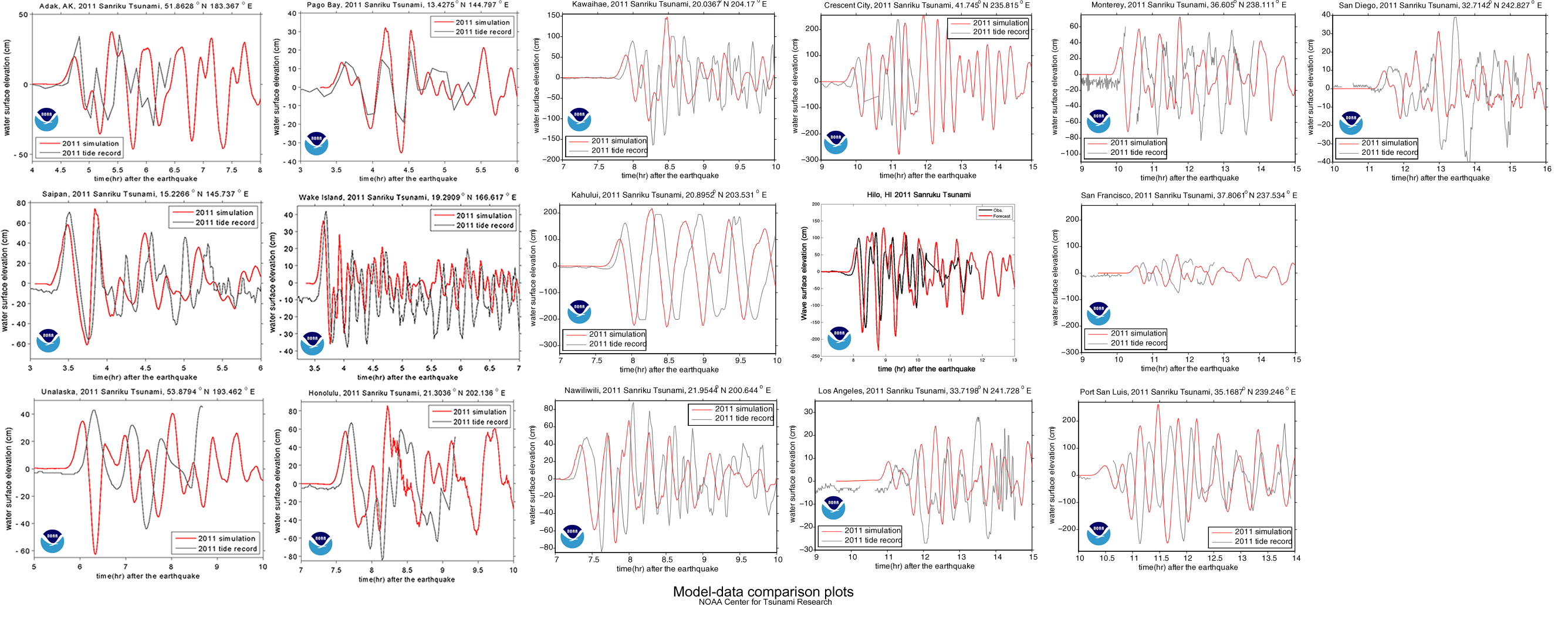
This is all very nice, a cute little exercise in algebra, but is it useful? Does it come anywhere close to reality? We can check by comparing it to actual measurements; the same ones used by NOAA to compare to their model (see here).

tsunami-model-data-honolulu — The red line is the tsunami's water height predicted by the NOAA computer models for Honolulu, Hawaii, while the black line is the actual water height, measured at a tidal gauge. Other comparisons can be found here.

680_20110311-TsunamiWaveHeight — Tsunami wave heights in the Pacific, as modeled by NOAA. Notice how the force of the tsunami is focused across the center of the Pacific.

The graph shows a maximum height of about 60 cm, which is about three times larger than our model. NOAA’s estimate is within 20% of the actual maximum heights, but they’ve spent a bit more time on this problem, so they should be a little better than us. You can find all the gruesome details on NOAA’s Center for Tsunami Research site’s Tsunami Forecasting page.

Notes

1. The maximum height of a tsunami depends on how much up-and-down motion was caused by the earthquake. ScienceDaily reports on a 2007 article that tried to figure out if you could predict the size of a tsunami based on the type of earthquake that caused it.

2. Using buoys in the area, NOAA was able to detect and warn about the Japanese earthquake in about 9 minutes. How do they know where to place the buoys? Plate tectonics.

buoys-warning — The locations of the buoys in NOAA's tsunami warning system.

Update

The equations starting with (7) did not have the 2 on the r_iw term. That has been corrected. Note that the numerical calculations were correct so they have not changed. – Thanks to Spencer and Claude for helping me catch that.

Social Loafing: Getting Groups to Work Well Together

PsyBlog has an excellent summary of the research on social loafing, the phenomena where people working in a group work less compared to when they work alone. Because we do so much group work, this is sometimes an issue.

The first research on social loafing came from Max Ringelmann way back in 1913 (Ringelmann, 1913). He had people pulling on a rope, and compared the maximum they could have pulled, based on individual test, to how much each person actually pulled. The results were, kind of, sad; with eight people, each one only pulled half as much as their maximum potential strength. A graph of Ringelmann’s data is shown below. If everyone pulled at their maximum the line would have stayed horizontal at 1.

ringelmann-data — The relative loafing of people working in a group. As the group gets larger, the amount of work per person decreases from its maximum of 1. Data from Ringelmann (1913)

The PsyBlog article points out three reasons why people tend to loaf in groups:

We expect others to loaf so we do it, too.
We feel more anonymous the larger the group, so we feel less need to put in the effort.
We often don’t have a clear idea about how much we need to contribute, so we don’t put in as much as we could.

This can be summed up in Latane’s Social Theory:

If a person is the target of social forces, increasing the number of other persons diminishes the relative social pressure on each person.

— Latane et al., 1979: Many hands make light the work: The causes and consequences of social loafing in the Journal of Personality and Social Psycology. Quote via Keith Rolag’s Website.

How do we deal with this

The key is making sure students are motivated to do the work. We want self-motivated students, but creating the right environment, especially by training students in how to work in a group will help.

Make sure students realize the importance of their work; this makes them more motivated.
Build group cohesion; team members contribute more if they value the group they’re in.
Make sure the group clearly and fairly divides the work. Let everyone be part of the decision making process so students have choices in what to do will help them be more invested in their part of the work.
Make sure each group member feels accountable for their share of the work.

A Brief Excursion into Mathematics

Ringelmann’s data falls on a remarkably straight line, so I used Excel to plot a trendline. As my algebra students know, you only need two points to write the equation of a line, however, Excel uses linear regression to get the best-fit line through all the data. Not all the data points will be on the line (sometimes none of them will be on the line) but the sum of the distance from each point to the line is minimized.

Curiously, since the data is pretty close to a straight line, you can extend the line to the x-axis to find out how many people it would take for no-one to be exerting any force at all. Students should be able to determine the equation of the line on their own, but you can get Excel to give you the equation of the trendline. From the plot we see:

y = -0.0732 x + 1.0707

At the x-axis, y = 0, so;

0 = -0.0732 x + 1.0707

solving for x we first subtract the constant, 1.0707 from both sides to get:

0 – 1.0707 = -0.0732 x + 1.0707 – 1.0707

giving:

-1.0707 = -0.0732 x

then divide by -0.0732 to isolate x:

$! \frac{-1.0707}{-0.0732} = \frac{-0.0732 x}{-0.0732}$

which yields:

x = 14.63

This means that with 15 people, no-one will be pulling on the rope. In fact, according to this equation, they’ll actually start pushing on the rope.

It’s an amazing result, but if you can find flaws with my argument or math, please let me know.

The Sound of π

A wonderful and facinating interpretation of what pi sounds like if you translate the first 33 digits into sounds.

Exercise on Wealth Distribution

Using the actual U.S. wealth distribution data from Norton and Arieli (2011; pdf), I created a little addendum to our exercise on the distribution of wealth.

I started with the definition of wealth. Students tend to think you’re referring to annual income, so I gave the example of someone who does not have a job but owns a house; they have no income but some wealth in the value of the house. Alternately, someone who has $2 million in the bank, but owes $4 million, actually has negative wealth.

Then I drew a little stick figure diagram to represent the population of the United States. With ten figures, paired up, that gives five parts, aka quintiles.

wealth-dist-example-01 — Breaking the population of the U.S. into five parts (quintiles) based on wealth. The least wealthy are to the right and the most wealthy are to the left.

Students were then presented with an empty bar graph and asked, “How much of the U.S.’s wealth is owned by the wealthiest 20% of the population?” Instead of asking in percentages (as are shown in the graph), I asked them to assume that the total wealth in the U.S. is $100 trillion.

wealth-dist-example-02 — Population with empty bar graph.

The first suggestion was $35 trillion, which is shown below. Others offered different amounts, ranging up to $50 trillion. Someone even suggested $15 trillion, which is not possible, since that would mean that the wealthiest 20% have less than 20% of the total wealth of the country.

wealth-dist-example-03 — If the wealthiest 20% owned 35% of the wealth of the U.S. the graph would look like this.

Once they got the idea, I showed them what the graph would look like in an idealized socialist country, where everyone had the same wealth.

wealth-dist-even — An even (socialist) distribution of wealth.

Finally, I asked my students to fill in what they believed to be the actual case for the U.S. for all five quintiles. The results had to add up to $100 trillion. They gave me their numbers individually before we broke up our meeting, and I entered it in the U.S. distribution of wealth spreadsheet to produce a graph.

After lunch, I showed them the results.

wealth-dist-all — Students' beliefs about the distribution of wealth in the U.S. (S1 through S10 and the average student response), compared to an equal distribution and the actual distribution (bottom).

For dramatic effect, I hid the last two bars at first. We talked over their numbers, then I showed them the equal distribution case (which they’d seen before), and finally the actual distribution.

wealth-dist-actual — Actual U.S. distribution of wealth. Data from Holder and Arieli (2011)

The response was salutary; a moment of surprised silence and then whispers. What then followed was a nice, short discussion. I pointed out the pie charts showing the U.S. versus an equal distribution, versus Sweden and asked what they would do, if they were an autocratic monarch, or if they were the president to make the U.S.’s distribution more equal.

How wealth is shared in the U.S. compared to and equal distribution (middle), compared to Sweden. Image adapted from Norton and Aireli (2011).

We talked about the government just taking private property, like the communists did. Then we talked about progressive taxation. We ended by talking about the estate tax, and meritocracy, which we’d touched on in the morning.

I thought the exercise worked very well. Not only did we get into an interesting economic issue, but got some practice with math and interpreting graphs too.

Beating probability

Since we just finished doing a bit of probabilities in math, here’s an article about how one guy figured out how to beat the lottery.

The first lottery Mohan Srivastava decoded was a tic-tac-toe game run by the Ontario Lottery in 2003. He was able to identify winning tickets with 90 percent accuracy.
–Lehrer (2010) in Cracking the Scratch Lottery Code

However, he decided not to just try to get rich of what he’d discovered. It’s an example of using the power of math for good:

“People often assume that I must be some extremely moral person because I didn’t take advantage of the lottery,” [Srivastava] says. “I can assure you that that’s not the case. I’d simply done the math and concluded that beating the game wasn’t worth my time.”

As a side note, my philosophy about the lottery is that it’s basically a tax on the poor:

[H]igh-frequency players tend to be poor and uneducated, which is why critics refer to lotteries as a regressive tax. (In a 2006 survey, 30 percent of people without a high school degree said that playing the lottery was a wealth-building strategy.)
–Lehrer (2010): Cracking the Scratch Lottery Code

Graphing discussion threads

wikipedia-threads — Graphic representation of the Wikipedia discussions about deleting articles. The image links to an interactive version of the graphic at http://notabilia.net .

Swings to the right are arguments for keeping the article, swings to the left are arguments to delete them. Moritz Stefaner and others’ website have created this wonderful graphic of Wikipedia’s discussion threads. They have lots more details and discussions on their website.

Graphing calculator pro. – Free app

Until tomorrow (Jan. 5th, 2011), the Graphing Calculator Pro iPod app is free (thanks Josh). It can do a lot, so it might take a minute figure out how to do the graphs and it can be a little fiddly (you can scale both axes separately, for example, which is nice unless you don’t intend to), but I like it. After just a couple of minutes, the student who found it was already playing with slopes.